1 Introduction
Time series refers to the process record of event changes and development in the order of time, which preserves the time structure of observation data. Therefore, time series are often studied and analyzed as a whole, rather than individual values. Data in many engineering fields exists in the form of time series, such as medical heart rate records, electrocardiograms, company financial statements, stock market prices, traffic congestion indexes, and the spread of epidemics, etc. These are typical time series sequence data. Time series has the characteristics of large data volume, high dimensionality, and real-time update. The main purposes of time series data analysis include prediction, clustering, classification (including anomaly detection), and correlation analysis. Among these tasks, the problem of time series classification has received much attention in existing related research [2].
Nowadays, with the continuous increase of time series data and the continuous deepening and expansion of analysis purposes, it is becoming more and more difficult to improve the accuracy of time series classification problems using traditional methods. However, in recent years, due to the continuous increase in the amount of data and calculations, deep learning has developed rapidly and has quickly become an important magic weapon for data research. Among them, the convolutional neural network (CNN) is the deepest learning model with the fastest development, the most mature technology, and the most successful application. From the classic LeNet[3], AlexNet[4], ResNet[5] to EfficentNet[6], the CNN network structure is constantly evolving. By sharing weights, CNN can greatly reduce the size of the model on the one hand, enabling rapid iteration of network optimization, on the other hand, it reduces the risk of over-fitting and has better generalization ability. These enable CNN to be successfully applied in many fields and have achieved great results, especially in the classification tasks in the image field.
Considering the difficulties faced by time series classification tasks and the great success of CNN in image classification tasks, researchers in related fields have put forward such a point of view: convert one-dimensional time series data into two-dimensional images, and convert time series classification tasks to Transform it into an image classification task, and then use the CNN model for training and learning. From a macro point of view, the classification task of time series is similar to the classification task of the image field. They both extract key features from the data and then classify them according to the features. It is this similarity that prompts the emergence of some new research, such as research on the method of converting time series data into two-dimensional images, research on the practical application of the conversion method to related fields, and so on. This paper will systematically review the methods of converting time series data into 2D images and its related applications, and finally analyze the advantages and disadvantages of each method with case studies.
2 Method overview
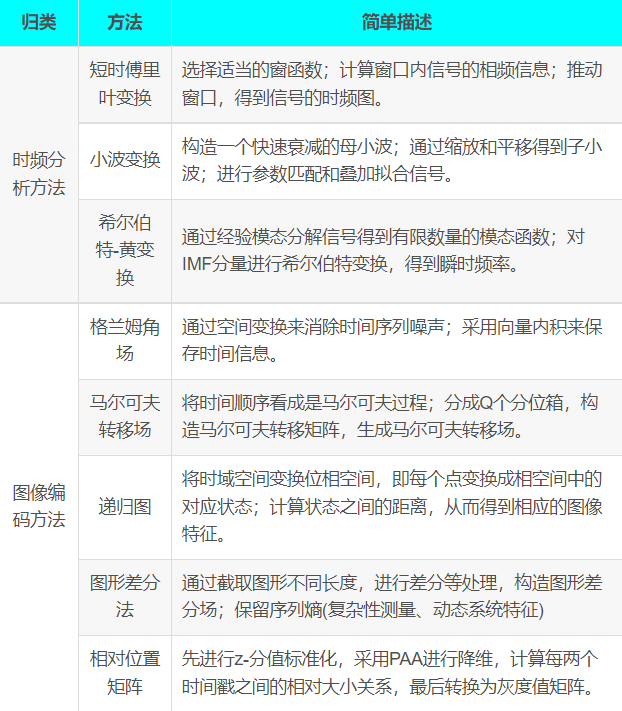
Images can be represented in the form of a matrix in a computer. Therefore, converting a time series to an image is equivalent to converting a time series to a matrix. According to this principle, as shown in Table 1, this paper organizes two categories of methods: the first category is time-frequency analysis method, which takes time series as the object of signal analysis, and uses time-frequency analysis method to analyze and solve its time-frequency diagram. There are short-time Fourier transform [7], wavelet transform [8], and Hilbert-Huang transform [9]; the second category is image coding method, which refers to time Sequences for image encoding mainly include Graham angle field [10], Markov transition field [10], recursive graph [11], graphic difference field [12], and relative position matrix [13]. The various methods are detailed below.
Table 1: Classification of time series to 2D image methods
2.1 Time-frequency analysis method
The time series is regarded as a signal whose frequency and phase change with time. According to the time-frequency analysis method, the time series data can be converted into a time-frequency diagram. The main methods are short-time Fourier transform, wavelet transform, and Hilber transform. Te-Huang transformation.
2.1.1 Short-time Fourier transform
See: Convert time series into images – short-time Fourier method Matlab implementation_vm-1215’s blog-CSDN blog
2.1.2 Wavelet transform
See: Convert time series into images – wavelet transform method Matlab implementation_vm-1215’s blog-CSDN blog
2.1.3 Hilbert-Huang Transformation
See: Convert time series into images – Hilbert-Huang transformation method Matlab implementation_vm-1215’s blog-CSDN blog
2.2 Image Coding Method
2.2.1 Graham Corner Field
See: Convert time series into images – Graham angle field method Matlab implementation_vm-1215’s blog-CSDN blog
2.2.2 Markov transfer field
See: Convert time series into images – Markov transfer field method Matlab implementation_vm-1215’s blog-CSDN blog
2.2.3 Recursive graphs
See: Convert time series into images – recursive graph method Matlab implementation_vm-1215’s blog-CSDN blog
2.2.4 Graph differential field
See: Convert time series into images – Graphical difference field method Matlab implementation_vm-1215’s blog-CSDN blog
2.2.5 Relative position matrix
See: Convert time series into images – relative position matrix method Matlab implementation_vm-1215’s blog-CSDN blog
3 Current status of applied research
Table 2: Application research of converting time series to 2D images
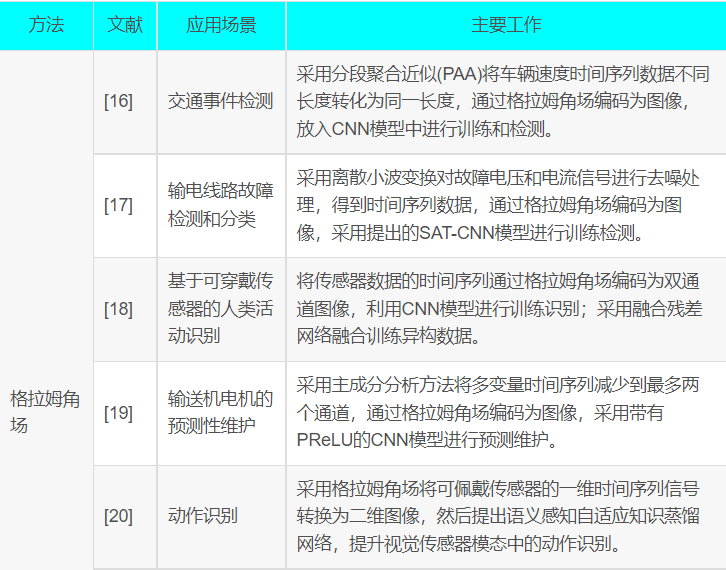
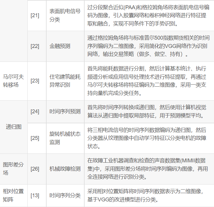
The purpose of converting time series data into two-dimensional images is to better extract features and achieve better performance. As shown in Table 2, it is the research status of relevant researchers applying this type of method in different fields in recent years. It mainly introduces the research scenarios, methods used and main work of each research. In various studies, the practical application of this type of method mainly has the following two problems:
There are various analysis tasks, such as classification, anomaly detection, prediction, etc. The length of the data to be analyzed may be different, and the size of the converted image may be different.
There are various scenarios in the form of time series data, such as mechanical status monitoring, finance, traffic flow, etc., so its attributes may have one type or multiple types.
For the above problems, there are mainly the following solutions:
Direct application of VS data preprocessing: some data itself has the same length, and the method of converting time series to two-dimensional images can be directly applied; while some data lengths are not the same, you can use segmentation aggregation approximation and other methods to unify the data length, and then proceed Image conversion. In addition, some data itself has a lot of noise, or other representative time series data features need to be extracted. In these cases, data preprocessing can be performed before applying this type of method.

Single-channel VS multi-channel: Each attribute of time series data can be converted into a graph through visualization, as a channel in the overall converted graph. Therefore, if there is only one attribute, it is transformed into a single-channel map; if there are multiple attributes, it is transformed into a multi-channel map. In addition, if there are too many types of attributes and the attributes are highly correlated, dimensionality reduction can also be performed by principal component analysis.

4 Method simulation and analysis
In order to further analyze the performance of different time series image conversion methods, all methods are implemented here one by one. As shown in Figure 1, there are two time series data. The data is the speed data of a certain section of the Guangzhou Airport Expressway for a certain period of time. The left picture shows the speed data under normal conditions, and the right picture shows the abnormal events. The speed data:
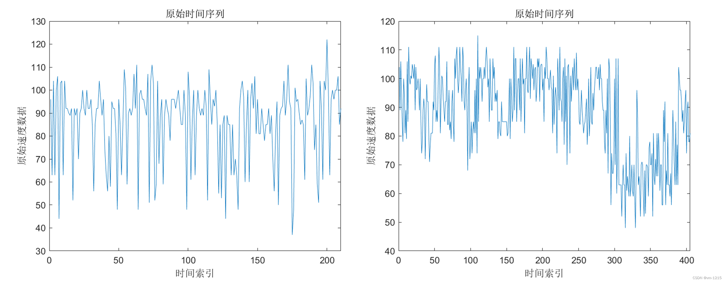
Figure 1: The left image shows the data under non-events, and the right image shows the data under events.
Using the methods described in detail above to convert time series to two-dimensional images, the time-frequency image conversion results are shown in Figure 2, and the image encoding conversion results are shown in Figure 3:
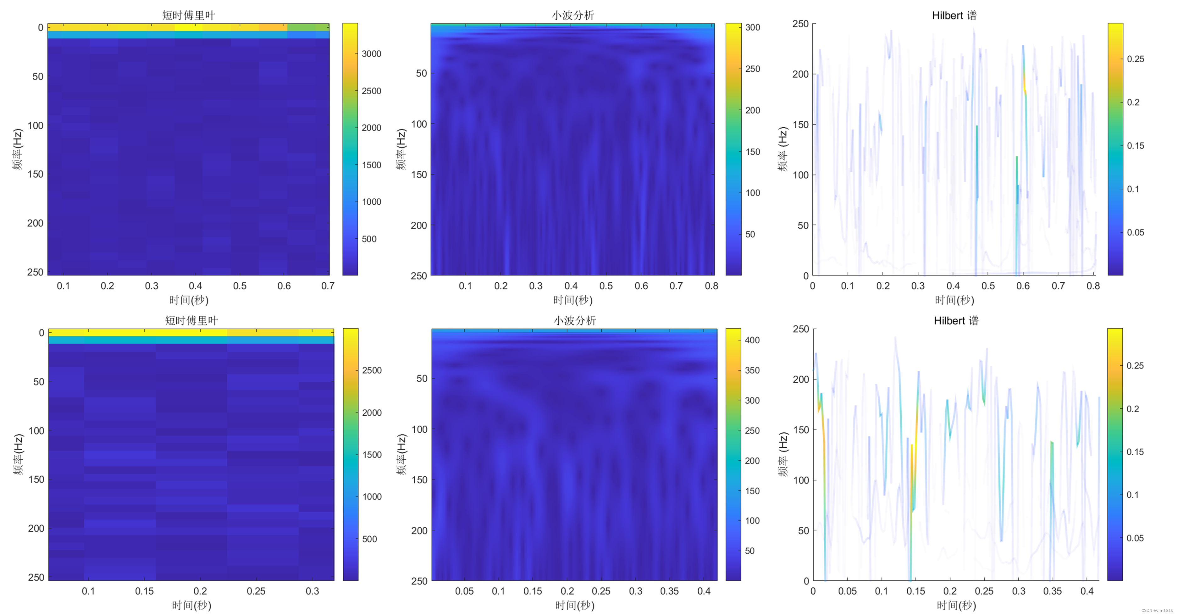
Figure 2: The result graph of the time-frequency graph conversion method, the first column is the graph under the abnormal scene, and the second column is the graph under the normal scene.
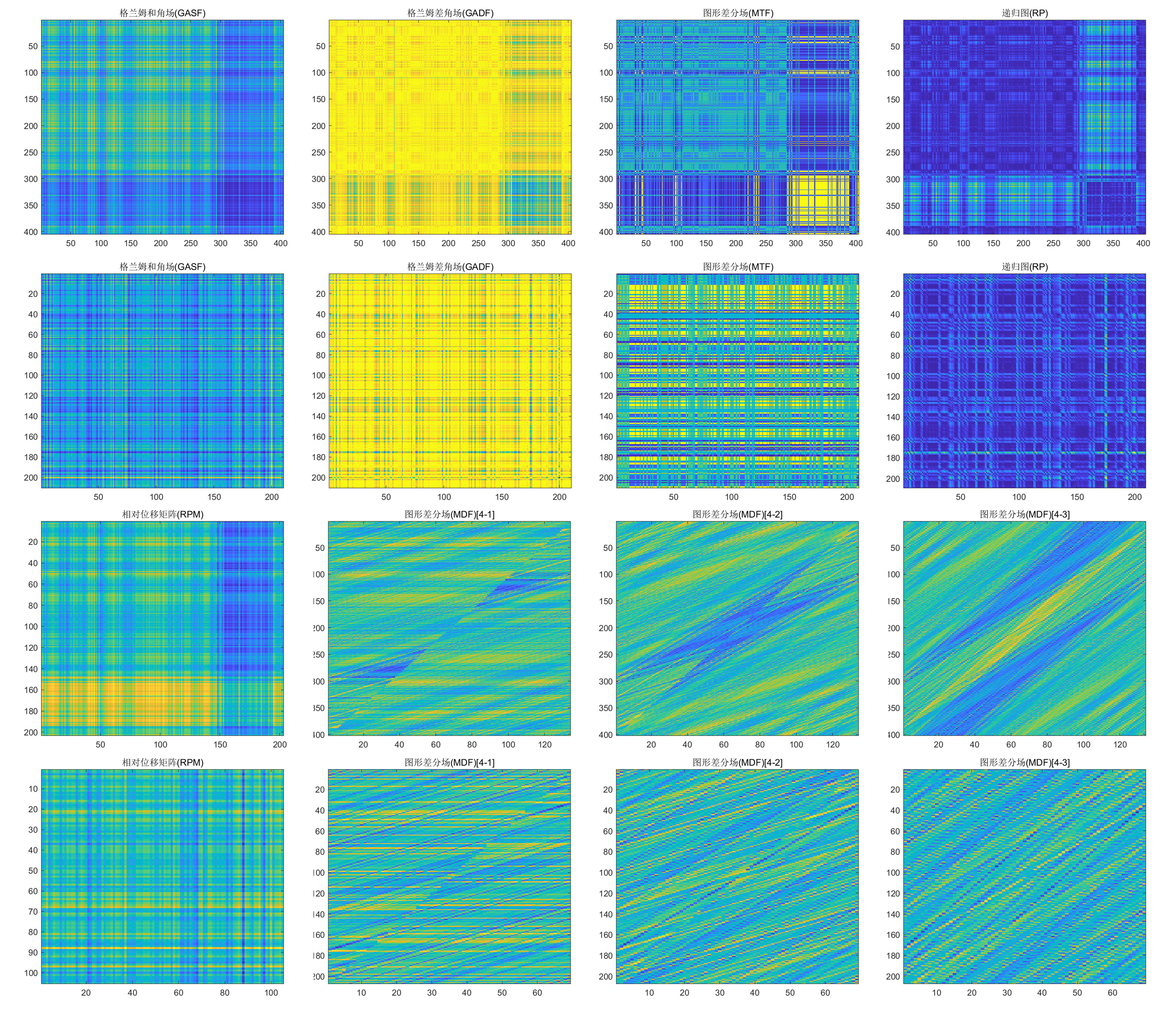
Figure 3: The result graph of the graph encoding conversion method, the first and third columns are the graphs under the abnormal scene, and the second and fourth columns are the graphs under the normal scene
It can be seen that the experimental results of the time-frequency method are very different from other methods, and there is no obvious difference in the experimental results of the time-frequency analysis method from the image. This is because the time-frequency analysis method analyzes the fluctuation frequency of the data, and the fluctuation frequency It is not an abnormal feature of the data; in contrast, other methods have obvious image features, and block abnormal features will appear, and the experimental results of GAF, MTF, RP, and RPM are similar.
Part of the code is:
import pandas as pd
import matplotlib.pyplot as plt
import numpy as np
import seaborn as sns
import math
def GAF(X):
”’
the code of GAF
input: the time series in raw
output: the heatmap of GASF and GADF
”’
# normalization to [-1,1]
X = ((X – np.max(X)) + (X – np.min(X))) / (np.max(X) + np.min(X))
# generate the GASF
gasf = X.T * X – np.sqrt(1 – np.square(X)).T * np.sqrt(1 – np.square(X))
sns.heatmap(gasf, cbar=False, square=True, cmap=’GnBu’,xticklabels=False, yticklabels=False)
# plt.show()
plt.savefig(‘picture/GASF_1.jpg’)
# generate the GADF
gadf = np.sqrt(1 – np.square(X)).T * X + X.T * np.sqrt(1 – np.square(X))
# plot the heatmap
sns.heatmap(gadf, cbar=False, square=True, cmap=’GnBu’, xticklabels=False, yticklabels=False)
# plt.show()
plt.savefig(‘picture/GADF_1.jpg’)
return 0
def MTF(X):
”’
the code of MTF
input: the time series in raw
output: the heatmap of MTF
”’
# normalization to [0,1]
X = (X – np.min(X)) / (np.max(X) – np.min(X))
# the length of X
Xlen = X.shape[1]
# design the number of bins
Q = 4
# compute the temp matrix X_Q
X_Q = np.ones([1, Xlen]) * 4
# print(X_Q)
temp = 0
threshold = np.zeros([1, Q])
for i in range(Q):
# print((Xlen * i / Q))
# print(np.sum(X < temp))
while np.sum(X < temp) < (Xlen * i / Q):
temp += 0.01
# print(threshold.shape)
threshold[0][i] = temp
X_Q[np.where(X<temp)] -= 1
# print(X_Q)
# print(threshold)
# generate the Markov matrix
sum_MM = np.zeros([4,4])
# compute the probability of Markov
for i in range(Xlen-1):
if X_Q[0][i] – X_Q[0][i+1] == -3:
sum_MM[0][3] = sum_MM[0][3] + 1
elif X_Q[0][i] – X_Q[0][i+1] == -2:
if X_Q[0][i] == 1:
sum_MM[0][2] = sum_MM[0][2] + 1
elif X_Q[0][i] == 2:
sum_MM[1][3] = sum_MM[1][3] +1
elif X_Q[0][i] – X_Q[0][i+1] == -1:
if X_Q[0][i] == 1:
sum_MM[0][1] = sum_MM[0][1] + 1
elif X_Q[0][i] == 2:
sum_MM[1][2] = sum_MM[1][2] + 1
elif X_Q[0][i] == 3:
sum_MM[2][3] = sum_MM[2][3] + 1
elif X_Q[0][i] – X_Q[0][i+1] == 0:
if X_Q[0][i] == 1:
sum_MM[0][0] = sum_MM[0][0] + 1
elif X_Q[0][i] == 2:
sum_MM[1][1] = sum_MM[1][1] + 1
elif X_Q[0][i] == 3:
sum_MM[2][2] = sum_MM[2][2] + 1
elif X_Q[0][i] == 4:
sum_MM[3][3] = sum_MM[3][3] + 1
elif X_Q[0][i] – X_Q[0][i+1] == 1:
if X_Q[0][i] == 2:
sum_MM[1][0] = sum_MM[1][0] + 1
elif X_Q[0][i] == 3:
sum_MM[2][1] = sum_MM[2][1] + 1
elif X_Q[0][i] == 4:
sum_MM[3][2] = sum_MM[3][2] + 1
elif X_Q[0][i] – X_Q[0][i+1] == 2:
if X_Q[0][i] == 3:
sum_MM[2][0] = sum_MM[2][0] + 1
elif X_Q[0][i] == 4:
sum_MM[3][1] = sum_MM[3][1] + 1
elif X_Q[0][i] – X_Q[0][i+1] == 3:
sum_MM[3][0] = sum_MM[3][0] + 1
W = sum_MM
W = W / np.sum(W,axis=1)
# print(W)
# generate the Markov Transform Field
mtf = np.zeros([Xlen, Xlen])
for i in range(Xlen):
for j in range(Xlen):
# print(X_Q[0][i])
mtf[i][j] = W[int(X_Q[0][i])-1][int(X_Q[0][j])-1]
mtf = (mtf – mtf.min()) / (mtf.max()- mtf.min()) * 4
# generate the heatmap
sns.heatmap(mtf,cbar=False,square=True,cmap=’GnBu’,xticklabels=False,yticklabels=False)
# plt.show()
plt.savefig(‘picture/MTF_1.jpg’)
return 0
def RP(X):
# normalization to [0,1]
X = (X – np.max(X)) / (np.max(X) + np.min(X))
Xlen = X.shape[1]
# convert to the phase space(第一元素是此时高度,第二个给元素为下一时刻的高度)
S = np.zeros([Xlen-1,2])
S[:,0] = X[0,:-1]
S[:,1] = X[0,1:]
# compute RRP matrix
R = np.zeros([Xlen-1,Xlen-1])
for i in range(Xlen-1):
for j in range(Xlen-1):
R[i,j] = sum(pow(S[i,:]-S[j,:],2))
# normalization to [0,4] of RP
R = (R – R.min()) / (R.max() – R.min()) * 4
# show the heatmap(bwr,coolwarm,GnBu)
sns.heatmap(R, cbar=False, square=True,cmap=’GnBu’,xticklabels=False,yticklabels=False)
# plt.show()
plt.savefig(‘picture/RP_1.jpg’)
return 0
def MDF(X,n):
# normalization to [0,1]
X = (X – np.max(X)) / (np.max(X) + np.min(X))
# compute the length of time series and the range of d
T = X.shape[1]
dMax = math.floor((T-1)/(n-1))
# initial the M,IMG
M = np.zeros([n,T-n+1,dMax])
# initial the dM,K
dM = np.zeros([n-1,T-n+1,dMax])
K = np.ones([n-1,T-n+1,dMax])
for d in range(dMax):
d = d + 1
# initial the s
s = np.zeros([T-(n-1)*d])
for i in range(T-(n-1)*d):
s[i] = i
for ImageIndex in range(n):
# print(s+ImageIndex*d)
s_index = (s+ImageIndex*d).astype(np.int16)
s = s.astype(np.int16)
# print(X[0,s_index])
M[ImageIndex,s,d-1] = X[0,s_index]
if ImageIndex >= 1:
# motif difference
dM[ImageIndex-1,s,d-1] = M[ImageIndex,s,d-1] – M[ImageIndex-1,s,d-1]
# K
K[ImageIndex-1,s,d-1] = np.zeros([T-(n-1)*d])
IMG = np.zeros([n-1,T-n+1,dMax])
for ImageIndex in range(n-1):
# G
G = dM[ImageIndex]
# the rot180 of G
G_1 = G.reshape(1,(T-n+1)*dMax)
G_2 = G_1[0][::-1]
G_rot = G_2.reshape(T-n+1,dMax)
IMG[ImageIndex,:,:] = G + K[ImageIndex] * G_rot
sns.heatmap(IMG[ImageIndex,:,:].T, cbar=False, square=True, cmap=’GnBu’, xticklabels=False, yticklabels=False)
# plt.show()
# print(IMG)
plt.savefig(‘picture/MDF’+’%d’%ImageIndex+’_1.jpg’)
return 0
if __name__ == “__main__”:
# get the data
data = pd.read_csv(filename)
# dataframe to numpy
data_numpy = data.values
# show the motif of the data
fig1 = plt.figure(1)
plt.plot(range(len(data_numpy)), data_numpy)
plt.xlim([0, len(data_numpy)-1])
plt.ylim([20, 120])
plt.ylabel(‘speed’)
plt.xlabel(‘time index’)
plt.title(‘time series of normal’)
# plt.show()
plt.savefig(‘picture/normal.jpg’)
# GAF(data_numpy.T)
# MTF(data_numpy.T)
# RP(data_numpy.T)
n = 4
MDF(data_numpy.T,n)
# x=list()
# temp = list()
# for t in np.arange(0,10,0.01):
# temp.append(t)
# x.append(math.sin(t))
# print(x)
# plt.plot(temp,x)
# plt.show()
5 Summary and Analysis
This paper introduces in detail the current method of converting time series to two-dimensional images and its application status; at the same time, it takes the traffic anomaly detection scene as an example to analyze each method. The results of various studies show that converting time series data into two-dimensional images and using mature computer vision technology for feature extraction and recognition can effectively improve the effect, which will help the research of time series data. In general, the reason why such methods are better than traditional time series analysis methods is mainly due to the following points:
The transformation process is essentially a dimension-enhancing process, which means an increase in the amount of information, such as an increase in the relationship between data values at different times;
The transformation process is also a data processing process, which highlights the main characteristics of the data;
Efficient feature extraction can be performed with the help of feature extraction mechanisms in the field of computer vision;
Nowadays, with the continuous improvement of data acquisition technology and the extensive deployment of data acquisition equipment, time series data in many scenarios are emerging in large quantities, and efficient data analysis methods are urgently needed. It is a new breakthrough to transform the time series into two-dimensional images and analyze them with the help of existing research results in the field of images. There are still some research points to be explored in this field, such as the problem of not losing data during the conversion process. At present, compared with the image field, the field of time series analysis has not made a major breakthrough in the research progress. I hope this paper can provide a new perspective for researchers in related fields.
