
1. Main contributions
It is mainly the collection of some existing tricks and the module reparameterization and dynamic label assignment strategy, and finally the speed and accuracy in the range of 5 FPS to 160 FPS exceed all known target detectors.
The main optimization direction of current target detection: faster and stronger network architecture; more effective feature integration method; more accurate detection method; more accurate loss function; more effective label assignment method; more effective training method.
2. Main ideas
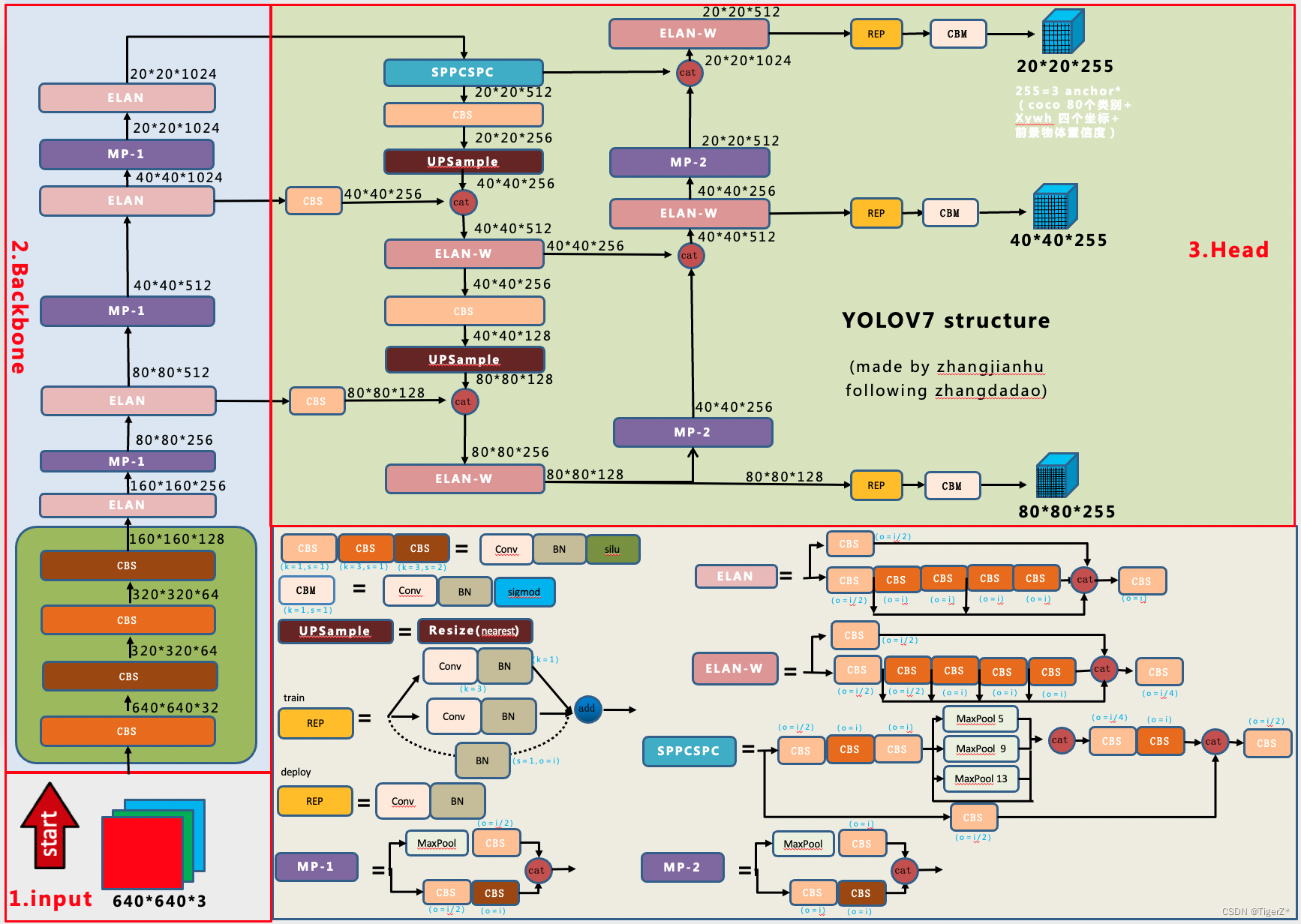
According to the paper, the yolov7 model (the corresponding open source git version is version 0.1) is currently more balanced in model accuracy and inference performance. According to the source code + exported onnx file + “Zhang Dao” and other network diagrams (modified some bugs that I think are present, and added some details). The very detailed network structure of yoloV7 version 0.1 has been redrawn. Notice:
1) The feature map result dimension annotation is in accordance with the flow direction of the arrow, not the fixed up and down direction.
2) The input and output only refers to the input and output of the current module, and the final result needs to be multiplied and calculated according to the flow direction as a whole.
3) This model version does not have an auxiliary training head.
On the whole, it is similar to YOLOV5, mainly the replacement of internal components of the network structure (involving some new sota design ideas), auxiliary training heads, label assignment ideas, etc. For overall preprocessing, loss, etc., please refer to yolov5: Target Detection Algorithm——YOLOV5_TigerZ*’s Blog-CSDN Blog_Target Detection yolov5
3. Specific details
1) input
The preprocessing method and related source code of YOLOV5 are reused as a whole. The only thing to note is that the official training and testing are mainly carried out on relatively large pictures such as 640*640 and 1280*1280.
For details, refer to the “Details” -> ‘input’ chapter in my other YOLOV5 blog. Target Detection Algorithm – YOLOV5_TigerZ*’s Blog – CSDN Blog_ Target Detection yolov5
2) backbone
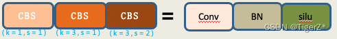
It mainly uses ELAN (this version of the model does not use the most complex E-ELAN structure mentioned in the paper) and MP structure. The activation function of this version of the model uses Silu.
For details, please refer to the cfg/training/yolov7.yaml file of the source code + models/yolo.py file + use export.py to export the onnx structure and use netron and other software to sort it out.
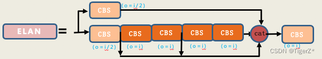
a. ELAN structure
By controlling the shortest and longest gradient paths, deeper networks can learn and converge efficiently. The author proposes the ELAN structure. E-ELAN based on ELAN design uses expand, shuffle, and merge cardinality to realize the ability to continuously enhance the network learning ability without destroying the original gradient path. (PS: This version of the model and the feedback from E6E netizens have not implemented E-ELAN). The relevant diagrams in the paper are as follows, and the cross stage connection is actually 1*1 convolution:
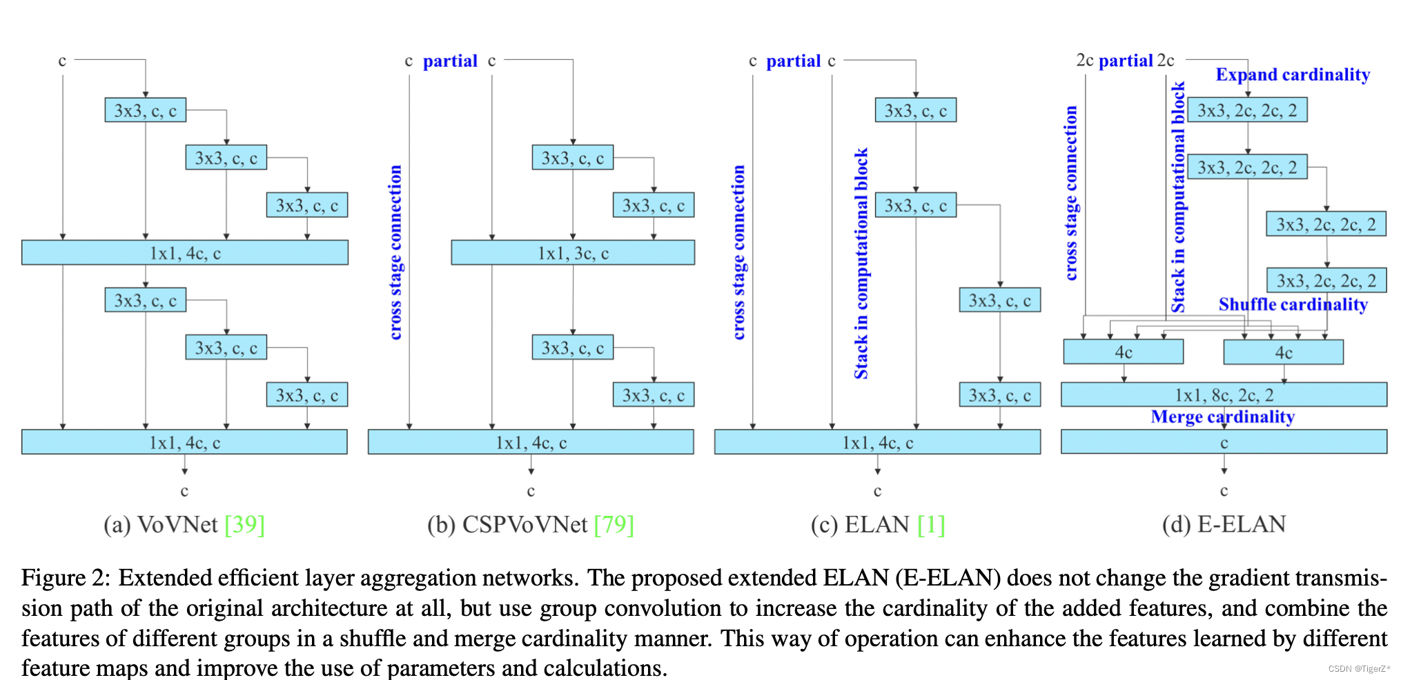
Simplified as follows:
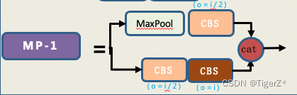
b. MP structure
I personally think that this is a relatively chicken thief structure. Before downsampling, we usually use maxpooling at the beginning, and then everyone chooses 3*3 convolution with stride = 2. Here the author gives full play to the principle of “children make choices, adults must”, and uses max pooling and conv with stride=2 at the same time. It should be noted that the number of channels before and after the MP in the backbone is unchanged.
3) neck & head
The overall structure of the detection head is similar to that of YOLOV5, and it is still an anchor based structure. It still does not use the decoupling head (classification and detection) idea of YOLOX and YOLOV6. This is not well understood at present, and it can be modified later if you have the energy. Mainly used:
*SPPCSPC structure
*ELAN-W (I named the unofficial name myself, because it is basically similar to ELAN, but it is not E-ELAN in the paper)
*MP structure (different from the backbone parameter)
*The more popular reparameterized structure Rep structure
For the above, please refer to the overall diagram in the “Main Ideas” in this blog, which contains these visualized components, which can be very intuitive to understand these structures. For details, please refer to the cfg/training/yolov7.yaml file of the source code + models/yolo.py file + use export.py to export the onnx structure and use netron and other software to sort it out.
4) loss function
There are mainly two types with and without auxiliary training heads, and the corresponding training scripts are train.py and train_aux.py.
Without an auxiliary training head (discussed in two parts: loss function and matching strategy).
loss function
The whole is consistent with YOLOV5, and is divided into three parts: coordinate loss, target confidence loss (GT is the ordinary iou in the training phase) and classification loss. The target confidence loss and classification loss use BCEWithLogitsLoss (binary cross-entropy loss with log), and the coordinate loss uses CIoU loss. For details, please refer to the ComputeLossOTA function in utils/loss.py to cooperate with the weight settings of each part in the configuration file.
matching strategy
It mainly refers to the popular simOTA used by YOLOV5 and YOLOV6.
S1. Before training, based on the gt frame in the training set, through the k-means clustering algorithm, 9 anchor frames arranged from small to large are obtained a priori. (optional)
S2. Match each gt with 9 anchors: Yolov5 calculates the ratio of its width to the width of the 9 anchors (the larger width is divided by the smaller width, the ratio is greater than 1, and the height below is the same), The ratio of height to height, in the two ratios of width ratio and height ratio, take the largest ratio. If this ratio is less than the set ratio threshold, the prediction frame of this anchor is called a positive sample. A gt may be matched with several anchors (maximum 9 at this time). Therefore, a gt may perform prediction training on different network layers, which greatly increases the number of positive samples. Of course, there will also be cases where gt does not match all anchors, so gt will be regarded as the background and will not participate in training. The size of the anchor box is not well designed.
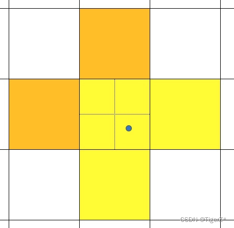
S3. Expand positive samples. According to the center position of the gt box, the nearest 2 neighborhood grids are also used as prediction grids, that is, a groundtruth box can be predicted by 3 grids; it can be found that the roughly estimated number of positive samples is increased compared to the previous yolo series tripled (maximum 27 matches at this point). The light yellow area in the figure below, where the solid line is the real grid of YOLO, and the dotted line is to divide a grid into four equal parts. Also as a positive sample.
S4. Obtain the prediction results with the top 10 maximum iou with the current gt. Sum the top10 (5-15, not sensitive) iou to get the k of the current gt. The minimum value of k is 1.
S5. Calculate the loss of each GT and candidate anchor according to the loss function (in the early stage, the classification loss weight will be increased, and the classification loss weight will be reduced later, such as 1:5->1:3), and the top K with the smallest loss will be retained.
S6. Remove the case where the same anchor is assigned to multiple GTs.
With an auxiliary training head (discussed in two parts: loss function and matching strategy).
In the paper, the Head responsible for the final output is called the lead Head, and the Head used for auxiliary training is called the auxiliary Head. This blog does not focus on the discussion, because the improvement of the structural experiments in the paper is relatively limited (0.3 points). For details, please refer to the original text.
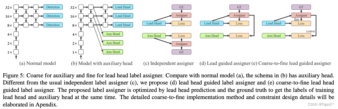
Some details: the loss function is the same as without the auxiliary head, and the weighting coefficient should not be too large (the ratio of aux head loss and lead head loss is 0.25:1), otherwise the accuracy of the results from the lead head will become lower. The matching strategy is only slightly different from the above without auxiliary headers (only lead head), among which auxiliary headers:
*If each grid in the lead head matches the gt, two surrounding grids will be added, and 4 grids will be added to the aux head (as shown in the second picture of the derivative above, a total of 5 grids in light yellow + orange are matched).
*In the lead head, the top10 samples iou are summed and rounded, while in the aux head, top20 is taken.
The aux head pays more attention to recall, while the lead head precisely selects samples from the aux head.
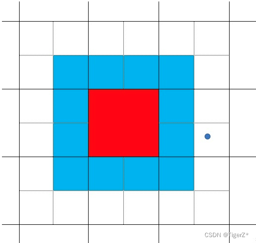
It should be noted that according to the center point regression method in yolov5, only the red feature grid in the picture can be predicted in the red + blue area in the picture (the grid composed of solid lines represents the feature map grid, and the dotted line represents a grid divided into 4 quadrant), it is impossible to predict the center point to gt (blue point)! And the red feature grid will be used as a positive sample during training. In the aux head, the model did not change the regression method for this situation. So in fact, in the aux head, even if the area assigned as a positive sample, after continuous learning, it may still not be able to fully fit to a particularly good effect.
5) trics
Overview: ELAN design ideas, MP dimensionality reduction components, Rep structure thinking, positive and negative sample matching strategies, auxiliary training head
6) inference
Test phase (non-training phase) process
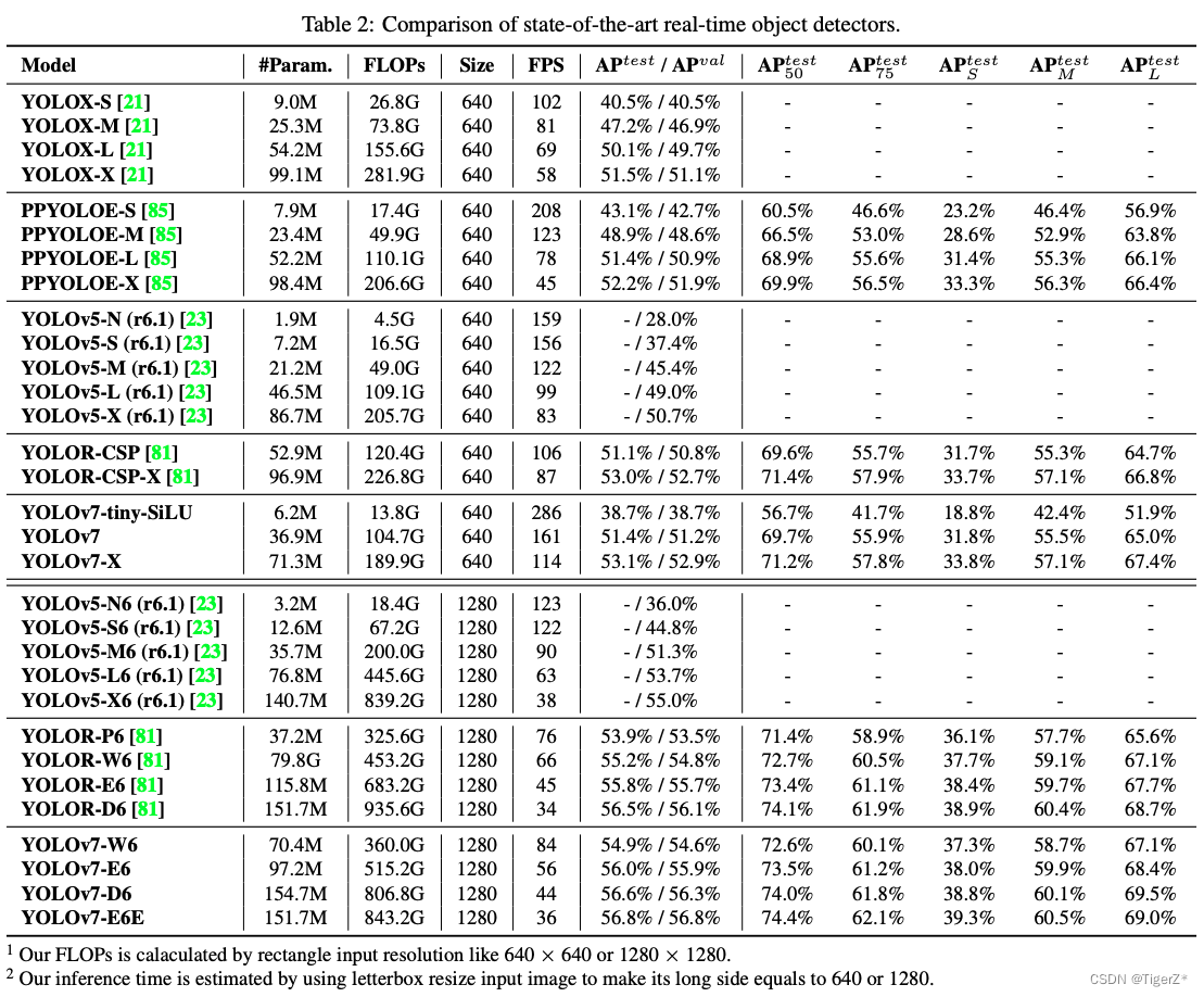
4. Results
reference connection
1. In-depth analysis of yolov7 network architecture_The invincible Zhang Dadao’s blog-CSDN blog
2. https://d246810g2000.medium.com/%E6%9C%80%E6%96%B0%E7%9A%84%E7%89%A9%E4%BB%B6%E5%81%B5%E6 %B8%AC%E7%8E%8B%E8%80%85-yolov7-%E4%BB%8B%E7%B4%B9-206c6adf2e69
3. [yolov7 Series 2] Positive and negative sample distribution strategy_The invincible Zhang Dadao’s blog-CSDN blog+
4. https://arxiv.org/pdf/2207.02696.pdf
5. Explain the basic network structure of Yolov7 in the Yolo series in a simple way bzdww
6. Understand the yolov7 network structure_athrunsunny’s blog-CSDN blog
7. The Yolov7 algorithm has made a comeback, and the accuracy and speed surpass all Yolo algorithms. The author of Yolov4 is a new masterpiece!
8. Explain the positive and negative sample distribution strategy of Yolov7 in simple terms
9. Detailed explanation of yolov7 positive and negative sample distribution bzdww
10. Jishi Developer Platform – Computer Vision Algorithm Development Platform