
Foreword: Since some unmanned driving-related projects and experiments may be done in the future, I learned some path planning algorithms during this period and wrote a matlab program for simulation. Starting this series is a summary of what I have learned, and I hope to learn more from the outstanding seniors.
1. Unmanned driving path planning
As we all know, unmanned driving can be roughly divided into three aspects of work: perception, decision-making and control.
Path planning is the decision-making stage between perception and control, and its main purpose is to provide vehicles with safe and collision-free paths to their destinations, taking into account vehicle dynamics, maneuverability, and corresponding rules and road boundary conditions.
The path planning problem can be divided into two aspects:
(1) Global path planning: The global path planning algorithm belongs to the static planning algorithm. It performs path planning based on the existing map information (SLAM), and finds an optimal path from the starting point to the target point. Usually, the implementation of global path planning includes classic algorithms such as Dijikstra algorithm, A* algorithm, and RRT algorithm, as well as intelligent algorithms such as ant colony algorithm and genetic algorithm;
(2) Local path planning: Local path planning is a dynamic programming algorithm. It is an unmanned vehicle that perceives the surrounding environment based on its own sensors and plans a route required for safe driving of a vehicle. It is often used in scenarios such as overtaking and obstacle avoidance. Usually, the realization of local path planning includes dynamic window algorithm (DWA), artificial potential field algorithm, Bezier curve algorithm, etc. Some scholars also propose intelligent algorithms such as neural network.
This series starts from the two aspects of unmanned driving path planning, introduces some classic algorithm principles, and puts forward some improvement suggestions based on some personal understanding and ideas, and simulates and verifies the algorithm through Matlab2019. If there are mistakes in the process, please leave a message in the comment area for discussion. If there is any infringement, please contact us in time.
So without further ado, let’s go directly to the introduction of the first part, the global path planning algorithm-RRT algorithm.
2. Global Path Planning – Principle of RRT Algorithm
The RRT algorithm, namely Rapid Random Tree algorithm (Rapid Random Tree), is an efficient path planning algorithm first proposed by LaValle in 1998. The RRT algorithm uses an initial root node to search in the space through random sampling, and then adds one leaf node after another to continuously expand the random tree. When the target point enters the random tree, the random tree expansion stops immediately, and a path from the starting point to the target point can be found at this time. The calculation process of the algorithm is as follows:
step1: Initialize the random tree. The starting point in the environment is used as the starting point of the random tree search. At this time, the tree contains only one node, the root node;
stpe2: random sampling in the environment. Randomly generate a point in the environment, if the point is not within the range of obstacles, calculate the Euclidean distance to all nodes in the random tree, and find the nearest node, if it is within the range of obstacles, regenerate and repeat the process until found ;
stpe3: generate new nodes. In the direction of the connection line, a new node is generated by pointing to a fixed growth distance, and it is judged whether the node is within the obstacle range. If it is not within the obstacle range, it will be added to the random tree. Otherwise, return to step2 to re-do the environment random sampling;
step4: Stop searching. When the distance to the target point is less than the set threshold, it means that the random tree has reached the target point, and will be added to the random tree as the last path node, and the algorithm ends and the planned path is obtained.
Due to its random sampling and probability completeness, the RRT algorithm has the following advantages:
(1) It does not need to model the environment specifically, and has strong spatial search capabilities;
(2) Fast path planning;
(3) It can well solve the path planning problem in complex environments.
But also because of the randomness, the RRT algorithm also has many deficiencies:
(1) The randomness is strong, the search is not targeted, there are many redundant points, and the paths generated by each planning are different, and not all of them are optimal paths;
(2) There may be problems such as complicated calculation, long time required, and easy to fall into dead zone;
(3) Since the expansion of the tree is connected between nodes, the final generated path is not smooth;
(4) It is not suitable for dynamic environments. When dynamic obstacles appear in the environment, the RRT algorithm cannot effectively detect them;
(5) For narrow and long terrain, it may not be possible to plan the path.
3. Realization of RRT algorithm in Matlab
Use matlab2019 to write the RRT algorithm, and some codes will be posted below for explanation.
1. Generate obstacles
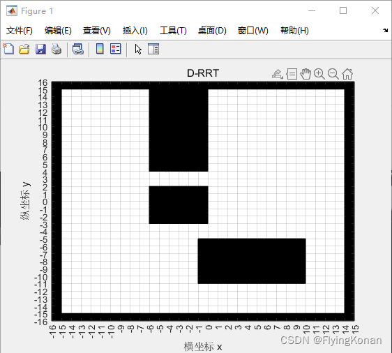
Simulate the grid map environment in matlab and customize the obstacle position.
%% 生成障碍物
ob1 = [0,-10,10,5]; % 三个矩形障碍物
ob2 = [-5,5,5,10];
ob3 = [-5,-2,5,4];
ob_limit_1 = [-15,-15,0,31]; % 边界障碍物
ob_limit_2 = [-15,-15,30,0];
ob_limit_3 = [15,-15,0,31];
ob_limit_4 = [-15,16,30,0];
ob = [ob1;ob2;ob3;ob_limit_1;ob_limit_2;ob_limit_3;ob_limit_4]; % 放到一个数组中统一管理
x_left_limit = -16; % 地图的边界
x_right_limit = 15;
y_left_limit = -16;
y_right_limit = 16;
I randomly choose to generate three rectangular obstacles here, and put them in the ob array for management, and define the boundaries of the map at the same time.
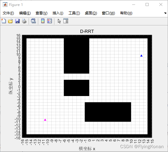
2. Initialize parameter settings
Initialize the obstacle expansion range, map resolution, robot radius, starting point, target point, growth distance and target point search threshold.
%% 初始化参数设置
extend_area = 0.2; % 膨胀范围
resolution = 1; % 分辨率
robot_radius = 0.2; % 机器人半径
goal = [-10, -10]; % 目标点
x_start = [13, 10]; % 起点
grow_distance = 1; % 生长距离
goal_radius = 1.5; % 在目标点为圆心,1.5m内就停止搜索
3. Initialize the random tree
Initialize the random tree, and define the tree structure tree to save the new node and its parent node, so that the planned path can be pushed back from the target point later.
%% 初始化随机树
tree.child = []; % 定义树结构体,保存新节点及其父节点
tree.parent = [];
tree.child = x_start; % 起点作为第一个节点
flag = 1; % 标志位
new_node_x = x_start(1,1); % 将起点作为第一个生成点
new_node_y = x_start(1,2);
new_node = [new_node_x, new_node_y];
4. The main function part
In the main function, a random point is first generated, and it is judged whether it is within the range of the map. If it is out of range, the flag position is set to 0.
rd_x = 30 * rand() – 15; % 生成随机点
rd_y = 30 * rand() – 15;
if (rd_x >= x_right_limit || rd_x <= x_left_limit ||… % 判断随机点是否在地图边界范围内
rd_y >= y_right_limit || rd_y <= y_left_limit)
flag = 0;
end
Call the function cal_distance to calculate the index of the node closest to the random point in the tree, and calculate the angle between the node and the random point and the positive direction of x.
[angle, min_idx] = cal_distance(rd_x, rd_y, tree); % 返回tree中最短距离节点索引及对应的和x正向夹角
The cal_distance function is defined as follows:
function [angle, min_idx] = cal_distance(rd_x, rd_y, tree)
distance = [];
i = 1;
while i<=size(tree.child,1)
dx = rd_x – tree.child(i,1);
dy = rd_y – tree.child(i,2);
d = sqrt(dx^2 + dy^2);
distance(i) = d;
i = i+1;
end
[~, min_idx] = min(distance);
angle = atan2(rd_y – tree.child(min_idx,2),rd_x – tree.child(min_idx,1));
end
Then generate new nodes.
new_node_x = tree.child(min_idx,1)+grow_distance*cos(angle);% 生成新的节点
new_node_y = tree.child(min_idx,2)+grow_distance*sin(angle);
new_node = [new_node_x, new_node_y];
Next, you need to judge the node:
① Whether the new node is within the range of obstacles;
② Whether the line segment between the new node and the parent node overlaps with the obstacle.
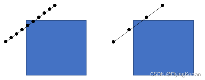
If any point is not satisfied, set the flag position to 0. In fact, the two judgments can be combined, that is, to judge whether the point on the line segment between the new node and the parent node is within the range of the obstacle.
for k=1:1:size(ob,1)
for i=min(tree.child(min_idx,1),new_node_x):0.01:max(tree.child(min_idx,1),new_node_x) % 判断生长之后路径与障碍物有无交叉部分
j = (tree.child(min_idx,2) – new_node_y)/(tree.child(min_idx,1) – new_node_x) *(i – new_node_x) + new_node_y;
if(i >=ob(k,1)-resolution && i <= ob(k,1)+ob(k,3) && j >= ob(k,2)-resolution && j <= ob(k,2)+ob(k,4))
flag = 0;
break
end
end
end
The method I use here is to write the straight line equation between the new node and the parent node, and then limit the change range of x to min(tree.child(min_idx,1),new_node_x) to max(tree.child(min_idx,1 ), new_node_x), 0.01 is the step size of the coordinate transformation. The smaller the step size is, the more accurate the judgment will be, but at the same time it will increase the amount of calculation; the larger the step size is, the faster the calculation speed is, but misjudgment is likely to occur, as shown in the figure below.
If the judgment flag is 1, you can add the new node to the tree, pay attention to save the new node and its parent node, and display it in the figure at the same time, and then reset the flag.
if (flag == true) % 若标志位为1,则可以将该新节点加入tree中
tree.child(end+1,:) = new_node;
tree.parent(end+1,:) = [tree.child(min_idx,1), tree.child(min_idx,2)];
plot(rd_x, rd_y, ‘.r’);hold on
plot(new_node_x, new_node_y,’.g’);hold on
plot([tree.child(min_idx,1),new_node_x], [tree.child(min_idx,2),new_node_y],’-b’);
end
flag = 1; % 标志位归位
The last step is to display obstacles, start and end points, etc. in the figure, and judge the distance from the new node to the target point. If it is less than the threshold, the search is stopped and the target point is added to the node, otherwise the process is repeated until the target point is found.
%% 显示
for i=1:1:size(ob,1) % 绘制障碍物
fill([ob(i,1)-resolution, ob(i,1)+ob(i,3),ob(i,1)+ob(i,3),ob(i,1)-resolution],…
[ob(i,2)-resolution,ob(i,2)-resolution,ob(i,2)+ob(i,4),ob(i,2)+ob(i,4)],’k’);
end
hold on
plot(x_start(1,1)-0.5*resolution, x_start(1,2)-0.5*resolution,’b^’,’MarkerFaceColor’,’b’,’MarkerSize’,4*resolution); % 起点
plot(goal(1,1)-0.5*resolution, goal(1,2)-0.5*resolution,’m^’,’MarkerFaceColor’,’m’,’MarkerSize’,4*resolution); % 终点
set(gca,’XLim’,[x_left_limit x_right_limit]); % X轴的数据显示范围
set(gca,’XTick’,[x_left_limit:resolution:x_right_limit]); % 设置要显示坐标刻度
set(gca,’YLim’,[y_left_limit y_right_limit]); % Y轴的数据显示范围
set(gca,’YTick’,[y_left_limit:resolution:y_right_limit]); % 设置要显示坐标刻度
grid on
title(‘D-RRT’);
xlabel(‘横坐标 x’);
ylabel(‘纵坐标 y’);
pause(0.05);
if (sqrt((new_node_x – goal(1,1))^2 + (new_node_y- goal(1,2))^2) <= goal_radius) % 若新节点到目标点距离小于阈值,则停止搜索,并将目标点加入到node中
tree.child(end+1,:) = goal; % 把终点加入到树中
tree.parent(end+1,:) = new_node;
disp(‘find goal!’);
break
end
5. Draw the optimal path
Starting from the target point, push back the planned path according to the node and parent node to the starting point in turn. Note that the length of the parent in the tree structure is 1 smaller than that of the child. Finally, the planned path is displayed in the figure.
%% 绘制最优路径
temp = tree.parent(end,:);
trajectory = [tree.child(end,1)-0.5*resolution, tree.child(end,2)-0.5*resolution];
for i=size(tree.child,1):-1:2
if(size(tree.child(i,:),2) ~= 0 & tree.child(i,:) == temp)
temp = tree.parent(i-1,:);
trajectory(end+1,:) = tree.child(i,:);
if(temp == x_start)
trajectory(end+1,:) = [temp(1,1) – 0.5*resolution, temp(1,2) – 0.5*resolution];
end
end
end
plot(trajectory(:,1), trajectory(:,2), ‘-r’,’LineWidth’,2);
pause(2);
The final effect of the program running is as follows:
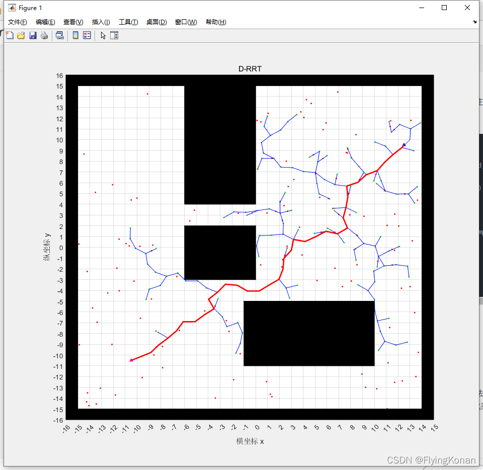
The red dots are random points at the generation point, the green dots are the nodes in the tree, and the red path is the path planned by the RRT algorithm.
6. Path smoothing (B-spline curve)
Since the planned path is connected by line segments, the path at the node is not smooth, which is also one of the disadvantages of the RRT algorithm. Generally speaking, there are many methods for trajectory smoothing, similar to Bezier curves, B-spline curves, etc. Here I use B-spline curve to smooth the planned path. I will explain the specific method and principle later when I have time. Here are the results first:
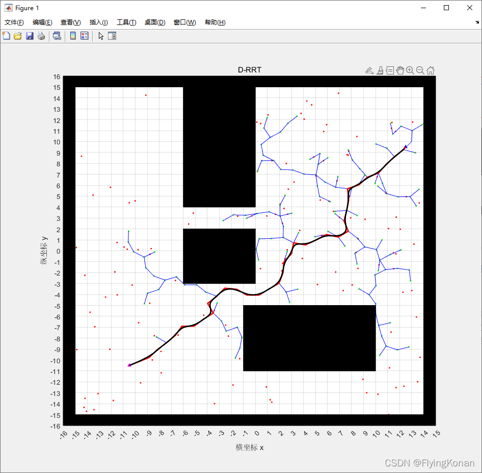
The black curve is the bit-smoothed path.
4. Comparison of multiple groups of results
① Comparison of two adjacent simulation results:
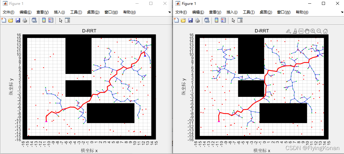
It can be seen that due to random sampling, the paths planned for any two times are different.
② Path planning in complex environments. Select a relatively complex environment, the simulation results are as follows:
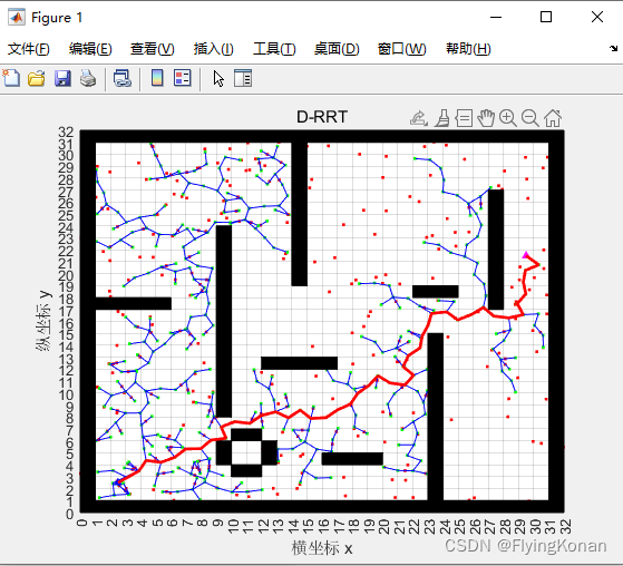
It can be seen that the RRT algorithm can well solve the path planning problem in complex environments.
③ Path planning under narrow passages. Select a narrow channel environment, the simulation results are as follows:
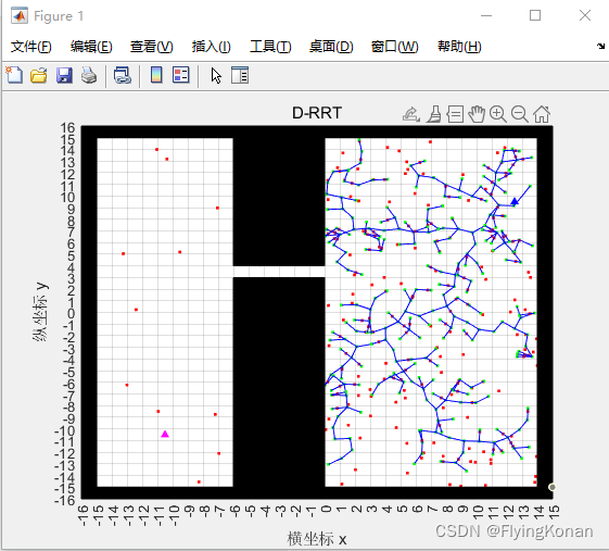
Due to the randomness of environment sampling, the probability of generating random points in the narrow channel is relatively low, which may lead to the failure to plan the path.
V. Conclusion
It can be seen from the final simulation results that the RRT algorithm can plan a path from the start point to the end point through random sampling of the space, and the planning speed is very fast, and it does not depend on the environment. However, the planning process is very random and has no purpose, and many redundant points will be generated, and the path planned each time is different, and it may not be possible to plan the path for narrow passages.