Foreword
This task is to use the ResNet18 network to practice a more general image classification task.
The ResNet series network, a well-known algorithm in the field of image classification, has been enduring for a long time, and it still has a wide range of research significance and application scenarios until today. It has been variously improved by the industry and is often used in image recognition tasks.
Today, I will mainly introduce the case of the ResNet-18 network structure, and other deep-level networks can be deduced by analogy.
ResNet-18, the number represents the depth of the network, that is to say, is the ResNet18 network 18 layers? In fact, 18 here specifies 18 layers with weights, including convolutional layers and fully connected layers, excluding pooling layers and BN layers.
Image classification (Image Classification) is a basic task in computer vision, which divides different images into different categories based on the semantics of images. Many tasks can also be converted to image classification tasks. For example, face detection is to judge whether there is a human face in an area, which can be regarded as a binary classification image classification task.
Dataset: The classic CIFAR-10 dataset in the field of computer vision used
Network layer: the network is a ResNet18 model
Optimizer: the optimizer is Adam optimizer
Loss function: The loss function is cross entropy loss
Evaluation index: The evaluation index is accuracy
Introduction to ResNet network:

two. data preprocessing
2.1 Dataset Introduction
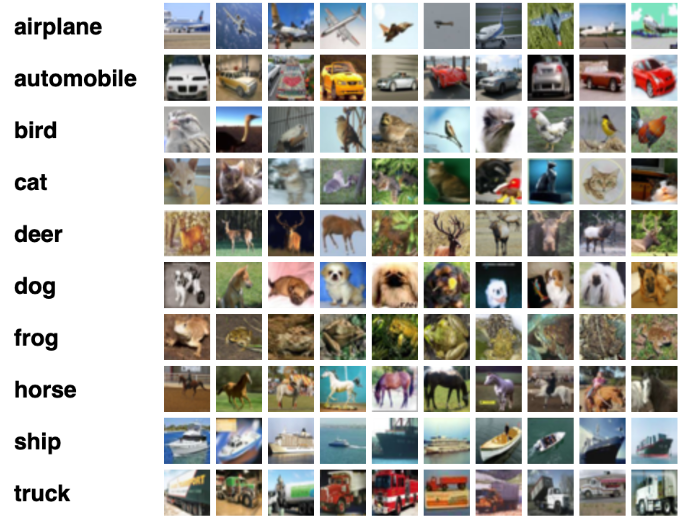
The CIFAR-10 data set contains 10 different categories, a total of 60,000 images, each of which has 6000 images, and the image size is 32×3232×32 pixels.
2.2 Data reading
In this experiment, the original training set was split into two parts, train_set and dev_set, including 40,000 and 10,000 samples respectively. Use data_batch_1 to data_batch_4 as the training set, data_batch_5 as the validation set, and test_batch as the test set. The final dataset is composed of:
Training set: 40,000 samples.
Validation set: 10,000 samples.
Test set: 10,000 samples.
The code to read a batch of data is as follows:
import os
import pickle
import numpy as np
def load_cifar10_batch(folder_path, batch_id=1, mode=’train’):
if mode == ‘test’:
file_path = os.path.join(folder_path, ‘test_batch’)
else:
file_path = os.path.join(folder_path, ‘data_batch_’+str(batch_id))
#加载数据集文件
with open(file_path, ‘rb’) as batch_file:
batch = pickle.load(batch_file, encoding = ‘latin1’)
imgs = batch[‘data’].reshape((len(batch[‘data’]),3,32,32)) / 255.
labels = batch[‘labels’]
return np.array(imgs, dtype=’float32′), np.array(labels)
imgs_batch, labels_batch = load_cifar10_batch(folder_path=’datasets/cifar-10-batches-py’,
batch_id=1, mode=’train’)
View the dimensions of the data:
#打印一下每个batch中X和y的维度
print (“batch of imgs shape: “,imgs_batch.shape, “batch of labels shape: “, labels_batch.shape)
batch of imgs shape: (10000, 3, 32, 32) batch of labels shape: (10000,)
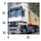
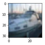
Visually observe one of the sample images and the corresponding labels, the code is as follows:
%matplotlib inline
import matplotlib.pyplot as plt
image, label = imgs_batch[1], labels_batch[1]
print(“The label in the picture is {}”.format(label))
plt.figure(figsize=(2, 2))
plt.imshow(image.transpose(1,2,0))
plt.savefig(‘cnn-car.pdf’)
2.3 Construct Dataset class
Construct a CIFAR10Dataset class, which will inherit from the paddle.io.DataSet class, and can process data one by one. The code is implemented as follows:
import paddle
import paddle.io as io
from paddle.vision.transforms import Normalize
class CIFAR10Dataset(io.Dataset):
def __init__(self, folder_path=’/home/aistudio/cifar-10-batches-py’, mode=’train’):
if mode == ‘train’:
#加载batch1-batch4作为训练集
self.imgs, self.labels = load_cifar10_batch(folder_path=folder_path, batch_id=1, mode=’train’)
for i in range(2, 5):
imgs_batch, labels_batch = load_cifar10_batch(folder_path=folder_path, batch_id=i, mode=’train’)
self.imgs, self.labels = np.concatenate([self.imgs, imgs_batch]), np.concatenate([self.labels, labels_batch])
elif mode == ‘dev’:
#加载batch5作为验证集
self.imgs, self.labels = load_cifar10_batch(folder_path=folder_path, batch_id=5, mode=’dev’)
elif mode == ‘test’:
#加载测试集
self.imgs, self.labels = load_cifar10_batch(folder_path=folder_path, mode=’test’)
self.transform = Normalize(mean=[0.4914, 0.4822, 0.4465], std=[0.2023, 0.1994, 0.2010], data_format=’CHW’)
def __getitem__(self, idx):
img, label = self.imgs[idx], self.labels[idx]
img = self.transform(img)
return img, label
def __len__(self):
return len(self.imgs)
paddle.seed(100)
train_dataset = CIFAR10Dataset(folder_path=’datasets/cifar-10-batches-py’, mode=’train’)
dev_dataset = CIFAR10Dataset(folder_path=’datasets/cifar-10-batches-py’, mode=’dev’)
test_dataset = CIFAR10Dataset(folder_path=’datasets/cifar-10-batches-py’, mode=’test’)
3. Model Construction
Image classification experiments using Resnet18 in the Paddle high-level API.
from paddle.vision.models import resnet18
resnet18_model = resnet18()
The high-level API of the flying paddle is a further package and upgrade of the flying paddle API, which provides a more concise and easy-to-use API, and further improves the ease of learning and use of the flying paddle. Among them, the flying paddle high-level API encapsulates the following modules:
The Model class supports the training of the model with only a few lines of code;
The image preprocessing module contains dozens of data processing functions, basically covering commonly used data processing and data enhancement methods;
Commonly used models in the field of computer vision and natural language processing, including but not limited to mobilenet, resnet, yolov3, cyclegan, bert, transformer, seq2seq, etc., also released pre-trained models of the corresponding models, you can use these models directly or here Based on the completion of secondary development.
4. Model Training
Reuse the RunnerV3 class, instantiate the RunnerV3 class, and pass in the training configuration. The training set and validation set are used for model training, and a total of 30 epochs are trained. In the experiment, the model with the highest accuracy is saved as the best model. The code is implemented as follows:
import paddle.nn.functional as F
import paddle.optimizer as opt
from nndl import RunnerV3, Accuracy
#指定运行设备
use_gpu = True if paddle.get_device().startswith(“gpu”) else False
if use_gpu:
paddle.set_device(‘gpu:0′)
#学习率大小
lr = 0.001
#批次大小
batch_size = 64
#加载数据
train_loader = io.DataLoader(train_dataset, batch_size=batch_size, shuffle=True)
dev_loader = io.DataLoader(dev_dataset, batch_size=batch_size)
test_loader = io.DataLoader(test_dataset, batch_size=batch_size)
#定义网络
model = resnet18_model
#定义优化器,这里使用Adam优化器以及l2正则化策略,相关内容在7.3.3.2和7.6.2中会进行详细介绍
optimizer = opt.Adam(learning_rate=lr, parameters=model.parameters(), weight_decay=0.005)
#定义损失函数
loss_fn = F.cross_entropy
#定义评价指标
metric = Accuracy(is_logist=True)
#实例化RunnerV3
runner = RunnerV3(model, optimizer, loss_fn, metric)
#启动训练
log_steps = 3000
eval_steps = 3000
runner.train(train_loader, dev_loader, num_epochs=30, log_steps=log_steps,
eval_steps=eval_steps, save_path=”best_model.pdparams”)
Visually observe the changes in the accuracy and loss of the training set and validation set.
from nndl import plot
plot(runner, fig_name=’cnn-loss4.pdf’)
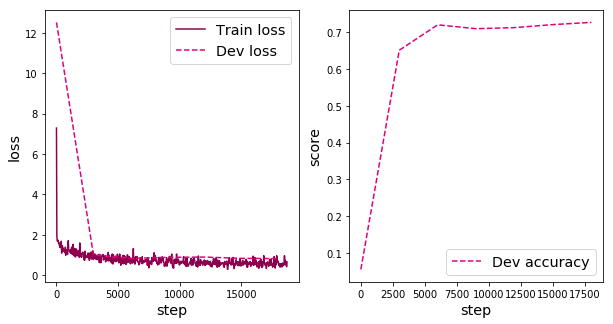
In this experiment, the Adam optimizer introduced in Chapter 7 is used for network optimization. If the SGD optimizer is used, it will cause over-fitting, and a good convergence effect cannot be obtained on the verification set. You can try to adjust the training configuration using other optimization strategies in Chapter 7 to achieve higher model accuracy.
5. Model evaluation
Use the test data to evaluate the best model saved during the training process, and observe the accuracy and loss of the model on the test set. The code is implemented as follows:
# 加载最优模型
runner.load_model(‘best_model.pdparams’)
# 模型评价
score, loss = runner.evaluate(test_loader)
print(“[Test] accuracy/loss: {:.4f}/{:.4f}”.format(score, loss))
[Test] accuracy/loss: 0.7234/0.8324
6. Model prediction
Similarly, you can also use the saved model to predict the data in the test set and observe the effect of the model. The specific code implementation is as follows:
#获取测试集中的一个batch的数据
X, label = next(test_loader())
logits = runner.predict(X)
#多分类,使用softmax计算预测概率
pred = F.softmax(logits)
#获取概率最大的类别
pred_class = paddle.argmax(pred[2]).numpy()
label = label[2][0].numpy()
#输出真实类别与预测类别
print(“The true category is {} and the predicted category is {}”.format(label[0], pred_class[0]))
#可视化图片
plt.figure(figsize=(2, 2))
imgs, labels = load_cifar10_batch(folder_path=’/home/aistudio/datasets/cifar-10-batches-py’, mode=’test’)
plt.imshow(imgs[2].transpose(1,2,0))
plt.savefig(‘cnn-test-vis.pdf’)
The true category is 8 and the predicted category is 8
True is 8, Predicted is 8. ship