1. Purpose of data indicator monitoring and attribution
Abnormal fluctuation of data indicators is one of the more common problems in the daily work of product operation and data analysis-related positions. Timely monitoring and early warning of abnormal fluctuations in core indicators can help businesses quickly locate and identify problems (attribution analysis), or capture business changes. information and seize market opportunities. Establishing a complete indicator anomaly monitoring and attribution scheme can improve the efficiency and accuracy of monitoring and attribution. This article mainly introduces the indicator anomaly monitoring and attribution scheme. hmi screen panel
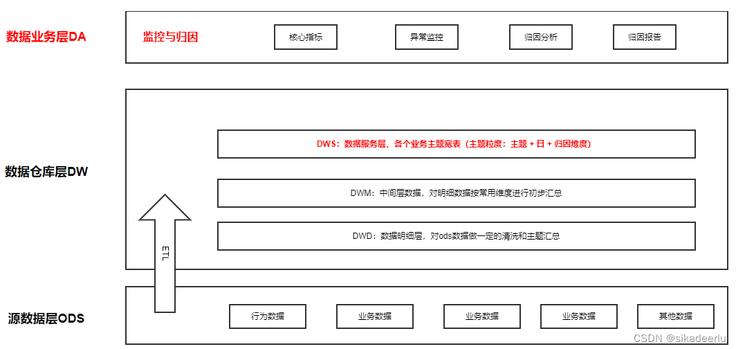
2. Monitoring and Attribution Framework
Monitoring and attribution are upper-level specific applications based on data warehouse construction. Indicator monitoring requires data in the dimensions of daily core indicators, and attribution requires data construction in the underlying dimension to be attributed. Appropriate modeling of the underlying data is monitoring. The first step of analysis.
The following figure is the framework of monitoring and attribution scheme based on data warehouse construction.

3. Indicator monitoring method and implementation
3.1 Indicator anomaly monitoring method
Here, the abnormal attribution method is explained by taking the APP daily activity indicator as an example.
1. Threshold method
a. Fixed threshold method: if the daily activity is greater than or less than a fixed value, an abnormality warning will be issued;
b. Same-cycle threshold method: if the daily activity fluctuates more than or less than a fixed percentage over the same period last week, an abnormal warning will be issued;
2. Statistical methods
a. 2/3 times standard deviation method: We know that in normal distribution , the probability of data distribution within 2 times standard deviation is 95.5%, and within 3 times the standard deviation probability is 99.7%, so if the daily life is greater than or less than 2 times the standard deviation of the daily average of one month (if the data has obvious weekly fluctuations, it can be pushed forward by week. If it is Friday, examine the mean and standard deviation of the first five Fridays and compare them), It can be considered that the data fluctuates abnormally.
b. 1.5 times IQR: Similar to the standard deviation, this method is based on boxplots for abnormal judgment.
3. Modeling method
First, model the indicators for prediction, and perform abnormal monitoring based on the deviation between the actual value and the predicted value. This method will be more flexible, and of course, it will take more time.
a. Time series method: There are two main methods for time series, one is the effect decomposition method, which mainly refers to the prophet method of facebook for modeling; the other is the prediction method ARIMA based on the statistical method of wide stationary time series, AR stands for autoregressive model , I stand for difference, MA stands for moving average model, and tsa.arima_model in statsmodel in python can make predictions.
b. Long Short-Term Memory Network LSTM
3.2 Sort out the core monitoring indicators and perform abnormal monitoring
1. Sort out the core business KPIs, such as daily activity and transaction volume, which are key indicators at the company level
2. Underlying data modeling for core indicators (summarization of daily dimension, summary of daily + attribution dimension)
3. Take 2 times the standard deviation as an example to judge whether it is abnormal: calculate the mean, standard deviation, and 2 times the standard deviation of the mean, standard deviation, and 2 times the standard deviation of the N days before the current date (or in a finer granularity, if the current date is Wednesday, the first N Wednesdays). What is the limit respectively, if the index of the day is outside the range of 2 times the standard deviation, it will be judged as abnormal fluctuation, and it will be checked whether the monitoring result is really abnormal, so as to continuously optimize the abnormal monitoring plan.
Four, abnormal attribution method and implementation
4.1 Introduction to the Principle of Root Cause Analysis of Adtributor
a. First calculate the ratio of the predicted value of each value to the overall predicted value in each dimension, and the ratio of the actual value of each value to the overall predicted value. Use the js divergence to calculate the difference between the predicted distribution and the actual distribution. The larger the js value, the the greater the difference
b. Calculate the proportion of the fluctuation of a factor in a certain dimension to the overall fluctuation, and arrange it in descending order
c. Sort the degree of difference, determine the dimension of the root cause, and give the explanatory power of each element within the dimension
4.2 Root cause analysis python code example of Adtributor
Taking the abnormal fluctuation of daily activities as an example, the root cause analysis is carried out. There are three data sets of the overall data of daily activities from March to May, and the daily activities are disassembled by city and model. The code below is the abnormal monitoring and root cause. Analyze the code.
############ 1、数据读取 ############
# 整体日活
data = pd.read_excel(‘./dau.xlsx’, sheet_name = ‘日活’)
dau_app = data[data[‘渠道’] == ‘App’]
# 按城市日活
data_city = pd.read_excel(‘./dau.xlsx’, sheet_name = ‘日活按城市拆分’)
dau_city_app = data_city[data_city[‘渠道’] == ‘App’]
# 按机型日活
data_manu = pd.read_excel(‘./dau.xlsx’, sheet_name = ‘日活按机型拆分’)
dau_manu_app = data_manu[data_manu[‘渠道’] == ‘App’]
############ 2、数据预处理 ############
# 添加星期
dau_app = dau_app.sort_values(by = [‘date’]) # 按照日期进行排序
dau_app[‘weekday’] = dau_app[‘date’].apply(lambda x: x.weekday() + 1) # 添加星期
dau_manu_app = dau_manu_app.sort_values(by = [‘date’]) # 按照日期进行排序
dau_manu_app[‘weekday’] = dau_manu_app[‘date’].apply(lambda x: x.weekday() + 1) # 添加星期
dau_city_app = dau_city_app.sort_values(by = [‘date’]) # 按照日期进行排序
dau_city_app[‘weekday’] = dau_city_app[‘date’].apply(lambda x: x.weekday() + 1) # 添加星期
############ 3、获取历史数据的均值、标准差信息 ############
# 定义函数:获取整体日活历史5周日活的均值、标准差信息
def get_his_week_dau_ms( currdate, xdaysbefcurr, currweek, dau_app):
thred = {} # 这里注意dict的赋值方式
dau_app_bef_35d = dau_app[(dau_app[‘date’] >= xdaysbefcurr) & (dau_app[‘date’] < currdate) & (dau_app[‘weekday’] == currweek)]
thred[‘deta’] = dau_app_bef_35d
thred[‘mean’] = dau_app_bef_35d[‘user_num1’].mean()
thred[‘std’] = dau_app_bef_35d[‘user_num1’].std()
thred[‘std_1_lower’] = dau_app_bef_35d[‘user_num1’].mean() – dau_app_bef_35d[‘user_num1’].std()
thred[‘std_1_upper’] = dau_app_bef_35d[‘user_num1’].mean() + dau_app_bef_35d[‘user_num1’].std()
thred[‘std_2_lower’] = dau_app_bef_35d[‘user_num1’].mean() – 2 * dau_app_bef_35d[‘user_num1’].std()
thred[‘std_2_upper’] = dau_app_bef_35d[‘user_num1’].mean() + 2 * dau_app_bef_35d[‘user_num1’].std()
thred[‘std_3_lower’] = dau_app_bef_35d[‘user_num1’].mean() – 3 * dau_app_bef_35d[‘user_num1’].std()
thred[‘std_3_upper’] = dau_app_bef_35d[‘user_num1’].mean() + 3 * dau_app_bef_35d[‘user_num1’].std()
return thred
# 定义函数:获取按城市日活历史5周日活的均值、标准差信息
def get_his_week_city_dau_ms( currdate, xdaysbefcurr, currweek, city, dau_app):
thred = {} # 这里注意dict的赋值方式
# 获取当前版本历史周对应的信息
dau_app_bef_35d = dau_app[(dau_app[‘date’] >= xdaysbefcurr) & (dau_app[‘date’] < currdate) & (dau_app[‘weekday’] == currweek) & (dau_app[‘$city’] == city)]
thred[‘deta’] = dau_app_bef_35d
thred[‘mean’] = dau_app_bef_35d[‘user_num1’].mean()
thred[‘std’] = dau_app_bef_35d[‘user_num1’].std()
thred[‘std_1_lower’] = dau_app_bef_35d[‘user_num1’].mean() – dau_app_bef_35d[‘user_num1’].std()
thred[‘std_1_upper’] = dau_app_bef_35d[‘user_num1’].mean() + dau_app_bef_35d[‘user_num1’].std()
thred[‘std_2_lower’] = dau_app_bef_35d[‘user_num1’].mean() – 2 * dau_app_bef_35d[‘user_num1’].std()
thred[‘std_2_upper’] = dau_app_bef_35d[‘user_num1’].mean() + 2 * dau_app_bef_35d[‘user_num1’].std()
thred[‘std_3_lower’] = dau_app_bef_35d[‘user_num1’].mean() – 3 * dau_app_bef_35d[‘user_num1’].std()
thred[‘std_3_upper’] = dau_app_bef_35d[‘user_num1’].mean() + 3 * dau_app_bef_35d[‘user_num1’].std()
return thred
# 定义函数:获取按机型日活历史5周日活的均值、标准差信息
def get_his_week_manu_dau_ms( currdate, xdaysbefcurr, currweek, manu, dau_app):
thred = {} # 这里注意dict的赋值方式
# 获取当前版本历史周对应的信息
dau_app_bef_35d = dau_app[(dau_app[‘date’] >= xdaysbefcurr) & (dau_app[‘date’] < currdate) & (dau_app[‘weekday’] == currweek) & (dau_app[‘$manufacturer’] == manu)]
thred[‘deta’] = dau_app_bef_35d
thred[‘mean’] = dau_app_bef_35d[‘user_num1’].mean()
thred[‘std’] = dau_app_bef_35d[‘user_num1’].std()
thred[‘std_1_lower’] = dau_app_bef_35d[‘user_num1’].mean() – dau_app_bef_35d[‘user_num1’].std()
thred[‘std_1_upper’] = dau_app_bef_35d[‘user_num1’].mean() + dau_app_bef_35d[‘user_num1’].std()
thred[‘std_2_lower’] = dau_app_bef_35d[‘user_num1’].mean() – 2 * dau_app_bef_35d[‘user_num1’].std()
thred[‘std_2_upper’] = dau_app_bef_35d[‘user_num1’].mean() + 2 * dau_app_bef_35d[‘user_num1’].std()
thred[‘std_3_lower’] = dau_app_bef_35d[‘user_num1’].mean() – 3 * dau_app_bef_35d[‘user_num1’].std()
thred[‘std_3_upper’] = dau_app_bef_35d[‘user_num1’].mean() + 3 * dau_app_bef_35d[‘user_num1’].std()
return thred
# 添加整体日活的波动信息
for index, row in dau_app.iterrows():
# print(row)
currdate = row[‘date’]
xdaysbefcurr = row[‘date’] – datetime.timedelta(days = 35)
currweek = row[‘weekday’]
# print(‘–‘, currdate, xdaysbefcurr, currweek)
tmp = get_his_week_dau_ms(currdate, xdaysbefcurr, currweek, dau_app)
dau_app.at[index, ‘his_mean’] = tmp[‘mean’]
dau_app.at[index, ‘his_std’] = tmp[‘std’]
dau_app.at[index, ‘std_1_lower’] = tmp[‘std_1_lower’]
dau_app.at[index, ‘std_1_upper’] = tmp[‘std_1_upper’]
dau_app.at[index, ‘std_2_lower’] = tmp[‘std_2_lower’]
dau_app.at[index, ‘std_2_upper’] = tmp[‘std_2_upper’]
dau_app.at[index, ‘std_3_lower’] = tmp[‘std_3_lower’]
dau_app.at[index, ‘std_3_upper’] = tmp[‘std_3_upper’]
# 添加按城市日活的历史波动信息
for index, row in dau_city_app.iterrows():
currdate = row[‘date’]
xdaysbefcurr = row[‘date’] – datetime.timedelta(days = 35)
currweek = row[‘weekday’]
city = row[‘$city’]
# print(‘–‘, currdate, xdaysbefcurr, currweek)
tmp = get_his_week_city_dau_ms(currdate, xdaysbefcurr, currweek, city, dau_city_app)
dau_city_app.at[index, ‘his_mean’] = tmp[‘mean’]
dau_city_app.at[index, ‘his_std’] = tmp[‘std’]
dau_city_app.at[index, ‘std_1_lower’] = tmp[‘std_1_lower’]
dau_city_app.at[index, ‘std_1_upper’] = tmp[‘std_1_upper’]
dau_city_app.at[index, ‘std_2_lower’] = tmp[‘std_2_lower’]
dau_city_app.at[index, ‘std_2_upper’] = tmp[‘std_2_upper’]
dau_city_app.at[index, ‘std_3_lower’] = tmp[‘std_3_lower’]
dau_city_app.at[index, ‘std_3_upper’] = tmp[‘std_3_upper’]
# 添加按机型日活的历史波动信息
for index, row in dau_manu_app.iterrows():
currdate = row[‘date’]
xdaysbefcurr = row[‘date’] – datetime.timedelta(days = 35)
currweek = row[‘weekday’]
manu = row[‘$manufacturer’]
# print(‘–‘, currdate, xdaysbefcurr, currweek)
tmp = get_his_week_manu_dau_ms(currdate, xdaysbefcurr, currweek, manu, dau_manu_app)
dau_manu_app.at[index, ‘his_mean’] = tmp[‘mean’]
dau_manu_app.at[index, ‘his_std’] = tmp[‘std’]
dau_manu_app.at[index, ‘std_1_lower’] = tmp[‘std_1_lower’]
dau_manu_app.at[index, ‘std_1_upper’] = tmp[‘std_1_upper’]
dau_manu_app.at[index, ‘std_2_lower’] = tmp[‘std_2_lower’]
dau_manu_app.at[index, ‘std_2_upper’] = tmp[‘std_2_upper’]
dau_manu_app.at[index, ‘std_3_lower’] = tmp[‘std_3_lower’]
dau_manu_app.at[index, ‘std_3_upper’] = tmp[‘std_3_upper’]
############ 4、判断是否异常 ############
def get_if_abnormal(x):
# print(x)
flag = 0 # 默认为0,即为正常波动
# 如果 历史均值 his_mean 不为nan ,且 当前日活在 2倍标准差之外,则为异常波动
if pd.isna(x[‘his_mean’]):
return flag
elif x[‘user_num1’] > x[‘std_2_upper’] or x[‘user_num1’] < x[‘std_2_lower’]:
flag = 1
return flag
dau_app[‘is_abnormal’] = dau_app.apply(lambda x: get_if_abnormal(x), axis = 1)
dau_app[dau_app[‘is_abnormal’] == 1] # 查看被标记为异常的数据
############ 5、Adtributor根因分析 ############
##### 5.1 定义函数:首先计算js散度所需要的两个值,预测值占比和实际值占比
def get_js_detail_info(row_dim, row_all):
js_detail = {}
# 计算该水平下实际值占整体值的比例
if pd.isna(row_dim.user_num1) or pd.isna(row_all.user_num1):
real_pct = None
else:
real_pct = row_dim.user_num1/row_all.user_num1
# 计算该水平下预测值占整体预测值的比例
if pd.isna(row_dim.his_mean) or pd.isna(row_all.his_mean):
pred_pct = None
else:
pred_pct = row_dim.his_mean/row_all.his_mean
# 计算该水平实际值-预测值 占 整体实际值-预测值的 比例
if pd.isna(row_dim.his_mean) or pd.isna(row_all.his_mean) or pd.isna(row_dim.user_num1) or pd.isna(row_all.user_num1):
diff_pct = None
else:
diff_pct = (row_dim.user_num1 – row_dim.his_mean)/(row_all.user_num1 – row_all.his_mean)
js_detail[‘real_pct’] = real_pct
js_detail[‘pred_pct’] = pred_pct
js_detail[‘diff_pct’] = diff_pct
return js_detail
# 按城市日活添加 实际占比 和 预测占比
for index, row in dau_city_app_copy.iterrows():
row_all = dau_app[dau_app[‘date’] == row.date]
row_all = pd.Series(row_all.values[0], index = row_all.columns) # dataframe类型转为series类型
js_detail = get_js_detail_info(row, row_all)
print(‘js_detail’, js_detail)
dau_city_app_copy.at[index, ‘real_pct’] = js_detail[‘real_pct’]
dau_city_app_copy.at[index, ‘pred_pct’] = js_detail[‘pred_pct’]
dau_city_app_copy.at[index, ‘diff_pct’] = js_detail[‘diff_pct’]
# 按机型日活添加 实际占比和预测占比
for index, row in dau_manu_app_copy.iterrows():
row_all = dau_app[dau_app[‘date’] == row.date]
row_all = pd.Series(row_all.values[0], index = row_all.columns) # dataframe类型转为series类型
js_detail = get_js_detail_info(row, row_all)
print(‘js_detail’, js_detail)
dau_manu_app_copy.at[index, ‘real_pct’] = js_detail[‘real_pct’]
dau_manu_app_copy.at[index, ‘pred_pct’] = js_detail[‘pred_pct’]
dau_manu_app_copy.at[index, ‘diff_pct’] = js_detail[‘diff_pct’]
##### 5.2 定义函数计算js散度
def get_js_divergence(p, q):
p = np.array(p)
q = np.array(q)
M = (p + q)/2
js1 = 0.5 * np.sum(p * np.log(p/M))+ 0.5 *np.sum(q* np.log(q/M)) # 自己计算
js2 = 0.5 * stats.entropy(p, M) + 0.5 * stats.entropy(q, M) # scipy包中方法
print(‘js1’, js1)
print(‘js2’, js2)
return round(float(js2),4)
##### 5.3 以4月24日日活波动异常为例从城市和机型维度进行归因
tmp = dau_city_app_copy[dau_city_app_copy[‘date’] == ‘2022-04-24’].dropna()
get_js_divergence(tmp[‘real_pct’], tmp[‘pred_pct’])
# js1: 0.014734253529123373 js2: 0.013824971768932472
tmp2 = dau_manu_app_copy[dau_manu_app_copy[‘date’] == ‘2022-04-24’].dropna()
get_js_divergence(tmp2[‘real_pct’], tmp2[‘pred_pct’])
# js1: 6.915922987763717e-05 js2: 6.9049339769412e-05 (约0.00010)
# 由此得出城市维度是异常波动的原因,查看当天城市维度的明细数据
tmp.sort_values(by = ‘diff_pct’, ascending = False,)

From the data of the city dimension, it can be seen that the actual ratio of Beijing’s daily activities to the overall daily activities on April 24 was 0.0772, and the proportion was 0.0378 according to the prediction of historical data. The fluctuation of Beijing’s daily activities accounted for 29.20% of the overall daily activities. Combined with The recent epidemic situation is speculated to be mainly due to the business fluctuations caused by the recent repeated epidemics in Beijing.