1. Overview of Gaussian mixture model
A Gaussian mixture model (GMM) is a machine learning algorithm. They are used to classify data into different classes based on probability distributions. Gaussian mixture models can be used in many different fields, including finance, marketing, and more! Here is an introduction to Gaussian Mixture Models with real-world examples, what they do, and when you should use GMMs.
A Gaussian Mixture Model (GMM) is a probabilistic concept used to model real-world datasets. GMM is a generalization of the Gaussian distribution and can be used to represent any dataset that can be clustered into multiple Gaussian distributions.
A Gaussian mixture model is a probabilistic model that assumes that all data points are generated from a mixture of Gaussian distributions with unknown parameters.
Gaussian mixture models can be used for clustering, which is the task of grouping a set of data points into clusters. GMMs can be used to find clusters in a dataset that may not be well-defined. Additionally, GMMs can be used to estimate the probability that a new data point belongs to each cluster. Gaussian mixture models are also relatively robust to outliers, meaning that even if there are some data points that don’t fit perfectly into any cluster, they can still produce accurate results. This makes GMM a flexible and powerful data clustering tool. It can be understood as a probabilistic model where a Gaussian distribution is assumed for each group and they have means and covariances that define their parameters.
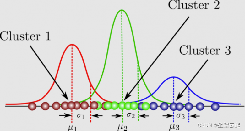
A GMM consists of two parts – a mean vector (μ) and a covariance matrix (Σ). A Gaussian distribution is defined as a continuous probability distribution with a bell-shaped curve. Another name for the Gaussian distribution is the normal distribution. Here is a picture of a Gaussian mixture model: it can be understood as a probabilistic model where a Gaussian distribution is assumed for each group, and they have a mean and covariance that define their parameters. A GMM consists of two parts – a mean vector (μ) and a covariance matrix (Σ). A Gaussian distribution is defined as a continuous probability distribution with a bell-shaped curve. Another name for the Gaussian distribution is the normal distribution. Here’s a picture of a Gaussian mixture model:
GMMs have many applications, such as density estimation, clustering, and image segmentation. For density estimation, GMMs can be used to estimate the probability density function for a set of data points. For clustering, GMMs can be used to group together data points from the same Gaussian distribution. For image segmentation, GMM can be used to divide the image into different regions.
Gaussian mixture models can be used for a variety of use cases, including identifying customer segments, detecting fraudulent activity, and clustering images. In each of these examples, the Gaussian mixture model was able to identify clusters in the data that might not be immediately obvious. Therefore, Gaussian mixture models are a powerful data analysis tool that should be considered for any clustering task.
In Gaussian mixture models, the expectation-maximization method is a powerful tool for estimating the parameters of a Gaussian mixture model (GMM). The expectation is called E, and the maximization is called M. Expect is used to find the Gaussian parameters used to represent each component of the Gaussian mixture model. Maximization is called M and it involves determining whether new data points can be added, you can read more about Expectation Maximization from the link below.
Here, we’ll explore Gaussian mixture models, an unsupervised technique for clustering and density estimation.
2. Mathematical principle of Gaussian mixture model
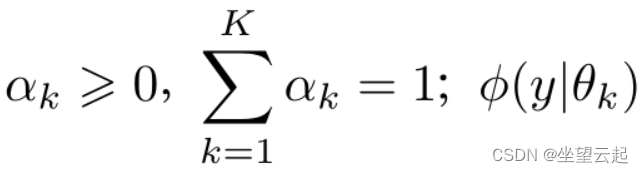
A Gaussian mixture model is a probability distribution model that has the following form,
The general mixture model can replace the Gaussian distribution density in the formula with any probability distribution density. We only introduce the most commonly used Gaussian mixture model.
3. Use Gaussian mixture model steps
Here are three different steps to use a Gaussian mixture model:
Determine the covariance matrix that defines how each Gaussian is related to each other. The more similar two Gaussian distributions are, the closer their means will be, and vice versa if they are far apart from each other in terms of similarity. Gaussian mixture models can have a diagonal or symmetric covariance matrix.
Determining the number of Gaussians in each group defines how many clusters there are.
Choose the hyperparameters that define how the Gaussian mixture model should be used to optimize the separated data, and whether the covariance matrix for each Gaussian should be diagonal or symmetric.
4. Differences from other clustering algorithms
Following are some of the main differences between Gaussian mixture models and the K-means algorithm used for clustering:
A Gaussian mixture model is a clustering algorithm that assumes that data points are generated from a mixture of Gaussian distributions with unknown parameters. The goal of the algorithm is to estimate the parameters of the Gaussian distributions, and the proportion of data points from each distribution. In contrast, K-means is a clustering algorithm that makes no assumptions about the underlying distribution of data points. Instead, it simply divides the data points into K clusters, where each cluster is defined by its centroid.
While Gaussian mixture models are more flexible, they can be more difficult to train than K-means. K-means generally converges faster, so may be preferred in cases where runtime is an important consideration.
In general, K-means is faster and more accurate when the dataset is large and the clusters are well separated. Gaussian mixture models are more accurate when the dataset is small or the clusters are not sufficiently separated.
Gaussian mixture models take into account the variance of the data, while K-means does not.
Gaussian mixture models are more flexible with respect to the shape of the clusters, while K-means is limited to spherical clusters.
Gaussian mixture models can handle missing data, while K-means cannot. This difference can make Gaussian mixture models more effective in certain applications, such as data with a lot of noise or data that is not well defined.
5. Suitable application scenarios
Gaussian mixture models can be used in a variety of scenarios, including when data are generated from a mixture of Gaussian distributions, when there is uncertainty about the correct number of clusters, and when clusters have different shapes. In each case, using a Gaussian mixture model can help improve the accuracy of the results. For example, when the data is generated by a mixture of Gaussian distributions, using a Gaussian mixture model can help better identify underlying patterns in the data. Additionally, using a Gaussian mixture model can help reduce error rates when there is uncertainty about the correct number of clusters.
Gaussian mixture models can be used for anomaly detection; by fitting a model to a dataset and then scoring new data points, points that are significantly different from the rest of the data (i.e., outliers) can be flagged. This is useful for identifying fraud or detecting errors in data collection.
In the case of time series analysis, GMM can be used to discover the relationship between volatility and trend and noise, which helps in predicting future stock prices. One cluster may contain trends in the time series, while another may contain noise and fluctuations from other factors, such as seasonality or external events affecting stock prices. To separate out these clusters, GMMs can be used as they provide probabilities for each class instead of simply splitting the data in two like K-means.
Another example is when there are different groups in the dataset and it is difficult to label them as belonging to one group or the other, which makes it difficult for other machine learning algorithms (such as K-means clustering algorithm) to separate the data. GMMs can be used in this case because they find the Gaussian Mixture Model that best describes each group and gives each cluster a probability which is helpful when labeling clusters.
Gaussian mixture models can generate synthetic data points similar to the original data and can also be used for data augmentation.
6. Practical Application Introduction
Here are some practical problems that can be solved using Gaussian Mixture Models:
Finding patterns in medical datasets: GMMs can be used to segment images into categories based on image content, or to find specific patterns in medical datasets. They can be used to find groups of patients with similar symptoms, identify disease subtypes, and even predict outcomes. In a recent study, a Gaussian mixture model was used to analyze a dataset of over 700,000 patient records. The model was able to identify previously unknown patterns in the data, which could lead to better treatments for cancer patients.
Modeling natural phenomena: GMMs can be used to model natural phenomena where the noise is found to follow a Gaussian distribution. Such probabilistic modeling models rely on the assumption that there exists some continuum of underlying unobserved entities or attributes, and that each member is associated with measurements made at equidistant points over multiple observation sessions.
Customer Behavior Analysis: GMM can be used in marketing to perform customer behavior analysis to predict future purchases based on historical data.
Stock Price Forecasting: Another area where Gaussian Mixture Models are used is in finance where they can be applied to price time series of stocks. GMMs can be used to detect change points in time series data and help find turning points in stock prices or other market movements that are difficult to spot due to volatility and noise.
Gene expression data analysis: Gaussian mixture models can be used for gene expression data analysis. In particular, GMMs can be used to detect differentially expressed genes between two conditions and to identify which genes may contribute to a certain phenotype or disease state.
7. Outlier detection based on GMM
import numpy as np
import matplotlib.pyplot as plt
from scipy import stats
from sklearn.mixture import GaussianMixture as GMM
plt.style.use(‘seaborn’)
# 特定分布的一维数据
np.random.seed(2)
x = np.concatenate([np.random.normal(0, 2, 2000), np.random.normal(5, 5, 2000), np.random.normal(3, 0.5, 600)])
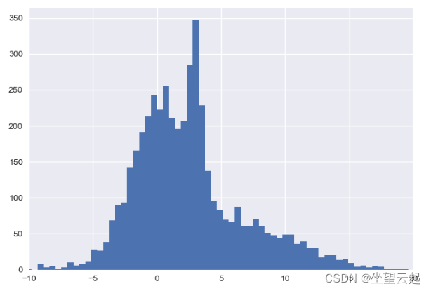
plt.hist(x, 80)
plt.xlim(-10, 20);
plt.show()
# 高斯混合模型将允许我们近似这个密度:
X = x[:, np.newaxis]
clf = GMM(4, max_iter=500, random_state=3).fit(X)
xpdf = np.linspace(-10, 20, 1000)
density = np.array([np.exp(clf.score([[xp]])) for xp in xpdf])
plt.hist(x, 80, density=True, alpha=0.5)
plt.plot(xpdf, density, ‘-r’)
plt.xlim(-10, 20)
plt.show()
plt.hist(x, 80, alpha=0.3)
plt.plot(xpdf, density, ‘-r’)
for i in range(clf.n_components):
pdf = clf.weights_[i] * stats.norm(clf.means_[i, 0], np.sqrt(clf.covariances_[i, 0])).pdf(xpdf)
plt.fill(xpdf, pdf, facecolor=’gray’, edgecolor=’none’, alpha=0.3)
plt.xlim(-10, 20)
plt.show()
np.random.seed(0)
# Add 20 outliers
true_outliers = np.sort(np.random.randint(0, len(x), 20))
y = x.copy()
y[true_outliers] += 50 * np.random.randn(20)
clf = GMM(4, max_iter=500, random_state=0).fit(y[:, np.newaxis])
xpdf = np.linspace(-10, 20, 1000)
density_noise = np.array([np.exp(clf.score([[xp]])) for xp in xpdf])
plt.hist(y, 80, density=True, alpha=0.5)
plt.plot(xpdf, density_noise, ‘-r’)
plt.xlim(-15, 30);
plt.show()
log_likelihood = np.array([clf.score_samples([[yy]]) for yy in y])
# log_likelihood = clf.score_samples(y[:, np.newaxis])[0]
plt.plot(y, log_likelihood, ‘.k’);
plt.show()
detected_outliers = np.where(log_likelihood < -9)[0]
print(“true outliers:”)
print(true_outliers)
print(“\ndetected outliers:”)
print(detected_outliers)